Module 7: Data Manipulation with tidyverse

Introduction

So far, we have learned how to:

create objects,
work with different data structures,
import data,
inspect datasets,
and visualize information.

But real datasets rarely arrive exactly in the format we need.

Before analyzing data, we often need to:

select variables,
filter observations,
rename columns,
create new variables,
count observations,
group data,
and calculate summaries.

This process is often called data manipulation or data wrangling.

In this module, we will use tools from the tidyverse, particularly the package dplyr, to manipulate our camera-trap data.

What is the tidyverse?

The tidyverse is a collection of R packages designed to work together for common data-science tasks.

We have already used some of them:

readr     → importing and exporting data

ggplot2   → data visualization

dplyr     → data manipulation

There are several others, but you do not need to learn all of them at once.

For this module, we will focus primarily on:

dplyr

When we load:

library(tidyverse)

the most commonly used tidyverse packages, including dplyr, are loaded automatically.

Let’s get started

Open your intro-r-course project and create a new R script.

Save it inside the scripts folder as:

module-07.R

Load the tidyverse:

library(tidyverse)

Then import our camera-trap record table:

recordTable <- read_csv(
  "data/recordTable.csv"
)

Let’s remind ourselves what the dataset looks like:

dim(recordTable)

[1] 3898   25

names(recordTable)

 [1] "RootFolder"        "File"              "RelativePath"     
 [4] "Station"           "Camera"            "DateTime"         
 [7] "Species"           "N_individuals"     "Sex"              
[10] "Age"               "Identifier"        "Comments"         
[13] "Favorite"          "DateTime_original" "year"             
[16] "date_shift"        "n_images"          "Date"             
[19] "Time"              "delta.time.secs"   "delta.time.mins"  
[22] "delta.time.hours"  "delta.time.days"   "DateTime2"        
[25] "Date2"

head(recordTable)

# A tibble: 6 × 25
  RootFolder       File  RelativePath Station Camera DateTime            Species
  <chr>            <chr> <chr>        <chr>   <chr>  <dttm>              <chr>  
1 Field Station 2… DSCF… "Control 0\… Contro… Contr… 2025-05-15 14:53:20 White-…
2 Field Station 2… DSCF… "Control 1\… Contro… Contr… 2025-06-05 04:25:19 Armadi…
3 Field Station 2… DSCF… "Control 1\… Contro… Contr… 2025-06-26 07:39:44 Armadi…
4 Field Station 2… DSCF… "Control 1\… Contro… Contr… 2025-06-26 08:07:20 Armadi…
5 Field Station 2… DSCF… "Control 1\… Contro… Contr… 2025-06-26 08:39:46 Armadi…
6 Field Station 2… DSCF… "Control 1\… Contro… Contr… 2025-07-20 01:11:11 Armadi…
# ℹ 18 more variables: N_individuals <dbl>, Sex <chr>, Age <chr>,
#   Identifier <chr>, Comments <chr>, Favorite <lgl>, DateTime_original <dttm>,
#   year <dbl>, date_shift <dbl>, n_images <dbl>, Date <date>, Time <time>,
#   delta.time.secs <dbl>, delta.time.mins <dbl>, delta.time.hours <dbl>,
#   delta.time.days <dbl>, DateTime2 <dttm>, Date2 <date>

Download the example data

If you do not already have the dataset from Module 5, you can download it here:

Download recordTable.csv

Think of `dplyr` as a set of verbs

Many dplyr functions are named after the action they perform.

Some of the most useful are:

Function	What does it do?
`select()`	Select columns
`filter()`	Select rows
`arrange()`	Sort rows
`rename()`	Rename columns
`mutate()`	Create or modify columns
`count()`	Count observations
`group_by()`	Create groups
`summarise()`	Calculate summaries

You will use these functions again and again when working with data in R.

Selecting columns with `select()`

Our recordTable contains many variables.

Sometimes we only need a few of them.

For example:

recordTable |>
  select(
    Station,
    Species,
    N_individuals,
    Age,
    n_images
  )

# A tibble: 3,898 × 5
   Station   Species           N_individuals Age     n_images
   <chr>     <chr>                     <dbl> <chr>      <dbl>
 1 Control 0 White-tailed deer             0 Unknown        1
 2 Control 1 Armadillo                     1 Adult          2
 3 Control 1 Armadillo                     2 Unknown        2
 4 Control 1 Armadillo                     1 Unknown        1
 5 Control 1 Armadillo                     1 Unknown        1
 6 Control 1 Armadillo                     1 Adult          2
 7 Control 1 Armadillo                     1 Adult          1
 8 Control 1 Bug                           1 Adult          1
 9 Control 1 Bug                           1 Adult          2
10 Control 1 Bug                           1 Adult          1
# ℹ 3,888 more rows

This creates a dataset containing only those columns.

We can save the result:

selected_records <- recordTable |>
  select(
    Station,
    Species,
    N_individuals,
    Age,
    n_images
  )

Now:

names(selected_records)

[1] "Station"       "Species"       "N_individuals" "Age"          
[5] "n_images"

contains only the columns we selected.

Removing columns

We can also use select() to remove columns.

For example:

recordTable |>
  select(
    -RootFolder,
    -RelativePath
  )

# A tibble: 3,898 × 23
   File     Station Camera DateTime            Species N_individuals Sex   Age  
   <chr>    <chr>   <chr>  <dttm>              <chr>           <dbl> <chr> <chr>
 1 DSCF000… Contro… Contr… 2025-05-15 14:53:20 White-…             0 <NA>  Unkn…
 2 DSCF013… Contro… Contr… 2025-06-05 04:25:19 Armadi…             1 Unkn… Adult
 3 DSCF042… Contro… Contr… 2025-06-26 07:39:44 Armadi…             2 Unkn… Unkn…
 4 DSCF042… Contro… Contr… 2025-06-26 08:07:20 Armadi…             1 Unkn… Unkn…
 5 DSCF042… Contro… Contr… 2025-06-26 08:39:46 Armadi…             1 Unkn… Unkn…
 6 DSCF040… Contro… Contr… 2025-07-20 01:11:11 Armadi…             1 Unkn… Adult
 7 DSCF041… Contro… Contr… 2025-07-20 02:11:12 Armadi…             1 Unkn… Adult
 8 DSCF016… Contro… Contr… 2025-06-09 13:26:30 Bug                 1 Unkn… Adult
 9 DSCF025… Contro… Contr… 2025-07-06 13:27:56 Bug                 1 Unkn… Adult
10 DSCF025… Contro… Contr… 2025-07-06 14:24:44 Bug                 1 Unkn… Adult
# ℹ 3,888 more rows
# ℹ 15 more variables: Identifier <chr>, Comments <chr>, Favorite <lgl>,
#   DateTime_original <dttm>, year <dbl>, date_shift <dbl>, n_images <dbl>,
#   Date <date>, Time <time>, delta.time.secs <dbl>, delta.time.mins <dbl>,
#   delta.time.hours <dbl>, delta.time.days <dbl>, DateTime2 <dttm>,
#   Date2 <date>

The - means:

Everything except these columns.

Selecting by data type

We can also select columns based on their type.

For example:

recordTable |>
  select(where(is.numeric))

# A tibble: 3,898 × 8
   N_individuals  year date_shift n_images delta.time.secs delta.time.mins
           <dbl> <dbl>      <dbl>    <dbl>           <dbl>           <dbl>
 1             0  2025         NA        1               0             0  
 2             1  2025         89        2               0             0  
 3             2  2025         89        2         1826065         30434. 
 4             1  2025         89        1            1656            27.6
 5             1  2025         89        1            1946            32.4
 6             1  2025         89        2         2046685         34111. 
 7             1  2025         89        1            3601            60  
 8             1  2025         89        1               0             0  
 9             1  2025         89        2         2332886         38881. 
10             1  2025         89        1            3408            56.8
# ℹ 3,888 more rows
# ℹ 2 more variables: delta.time.hours <dbl>, delta.time.days <dbl>

returns only numeric columns.

Tip

You do not need to memorize every option available in select().

Start with selecting columns by name. The more advanced selection tools become useful as your datasets become larger.

Filtering rows with `filter()`

While select() works with columns, filter() works with rows.

For example, let’s select only records of White-tailed deer:

deer_records <- recordTable |>
  filter(
    Species == "White-tailed deer"
  )

Check:

unique(deer_records$Species)

[1] "White-tailed deer"

All observations now correspond to the same species.

Filtering numeric values

We can also use relational operators.

For example, records containing more than one individual:

recordTable |>
  filter(
    N_individuals > 1
  )

# A tibble: 244 × 25
   RootFolder      File  RelativePath Station Camera DateTime            Species
   <chr>           <chr> <chr>        <chr>   <chr>  <dttm>              <chr>  
 1 Field Station … DSCF… "Control 1\… Contro… Contr… 2025-06-26 07:39:44 Armadi…
 2 Field Station … DSCF… "Control 1\… Contro… Contr… 2025-07-28 16:48:44 Bug    
 3 Field Station … DSCF… "Control 1\… Contro… Contr… 2025-07-29 15:10:02 Bug    
 4 Field Station … DSCF… "Control 1\… Contro… Contr… 2025-07-29 16:08:40 Bug    
 5 Field Station … DSCF… "Control 1\… Contro… Contr… 2025-07-30 15:38:00 Bug    
 6 Field Station … DSCF… "Control 1\… Contro… Contr… 2025-06-20 06:56:25 White-…
 7 Field Station … DSCF… "Control 1\… Contro… Contr… 2025-06-20 07:56:26 White-…
 8 Field Station … DSCF… "Control 1\… Contro… Contr… 2025-06-28 12:48:34 White-…
 9 Field Station … DSCF… "Control 2\… Contro… Contr… 2025-04-17 02:47:44 Armadi…
10 Field Station … DSCF… "Control 2\… Contro… contr… 2025-09-06 23:31:16 Bug    
# ℹ 234 more rows
# ℹ 18 more variables: N_individuals <dbl>, Sex <chr>, Age <chr>,
#   Identifier <chr>, Comments <chr>, Favorite <lgl>, DateTime_original <dttm>,
#   year <dbl>, date_shift <dbl>, n_images <dbl>, Date <date>, Time <time>,
#   delta.time.secs <dbl>, delta.time.mins <dbl>, delta.time.hours <dbl>,
#   delta.time.days <dbl>, DateTime2 <dttm>, Date2 <date>

Remember the operators we learned earlier:

>      greater than
>=     greater than or equal to
<      less than
<=     less than or equal to
==     equal to
!=     different from

Multiple filtering conditions

We can combine conditions.

For example:

recordTable |>
  filter(
    Species == "White-tailed deer",
    N_individuals > 1
  )

# A tibble: 86 × 25
   RootFolder      File  RelativePath Station Camera DateTime            Species
   <chr>           <chr> <chr>        <chr>   <chr>  <dttm>              <chr>  
 1 Field Station … DSCF… "Control 1\… Contro… Contr… 2025-06-20 06:56:25 White-…
 2 Field Station … DSCF… "Control 1\… Contro… Contr… 2025-06-20 07:56:26 White-…
 3 Field Station … DSCF… "Control 1\… Contro… Contr… 2025-06-28 12:48:34 White-…
 4 Field Station … DSCF… "Control 2\… Contro… Contr… 2025-04-24 15:32:46 White-…
 5 Field Station … DSCF… "Control 2\… Contro… Contr… 2025-04-24 16:55:22 White-…
 6 Field Station … DSCF… "Control 2\… Contro… Contr… 2025-05-05 14:58:46 White-…
 7 Field Station … DSCF… "Control 2\… Contro… contr… 2025-06-06 20:44:02 White-…
 8 Field Station … DSCF… "Control 2\… Contro… contr… 2025-06-06 21:44:04 White-…
 9 Field Station … DSCF… "Control 2\… Contro… contr… 2025-06-07 02:31:38 White-…
10 Field Station … DSCF… "Control 2\… Contro… contr… 2025-06-07 16:02:24 White-…
# ℹ 76 more rows
# ℹ 18 more variables: N_individuals <dbl>, Sex <chr>, Age <chr>,
#   Identifier <chr>, Comments <chr>, Favorite <lgl>, DateTime_original <dttm>,
#   year <dbl>, date_shift <dbl>, n_images <dbl>, Date <date>, Time <time>,
#   delta.time.secs <dbl>, delta.time.mins <dbl>, delta.time.hours <dbl>,
#   delta.time.days <dbl>, DateTime2 <dttm>, Date2 <date>

When conditions are separated by commas inside filter(), both conditions must be satisfied.

This is equivalent to using:

for AND.

We can also select several species using %in%.

recordTable |>
  filter(
    Species %in% c(
      "White-tailed deer",
      "Armadillo",
      "Racoon"
    )
  )

# A tibble: 2,342 × 25
   RootFolder      File  RelativePath Station Camera DateTime            Species
   <chr>           <chr> <chr>        <chr>   <chr>  <dttm>              <chr>  
 1 Field Station … DSCF… "Control 0\… Contro… Contr… 2025-05-15 14:53:20 White-…
 2 Field Station … DSCF… "Control 1\… Contro… Contr… 2025-06-05 04:25:19 Armadi…
 3 Field Station … DSCF… "Control 1\… Contro… Contr… 2025-06-26 07:39:44 Armadi…
 4 Field Station … DSCF… "Control 1\… Contro… Contr… 2025-06-26 08:07:20 Armadi…
 5 Field Station … DSCF… "Control 1\… Contro… Contr… 2025-06-26 08:39:46 Armadi…
 6 Field Station … DSCF… "Control 1\… Contro… Contr… 2025-07-20 01:11:11 Armadi…
 7 Field Station … DSCF… "Control 1\… Contro… Contr… 2025-07-20 02:11:12 Armadi…
 8 Field Station … DSCF… "Control 1\… Contro… Contr… 2025-06-07 23:35:55 Racoon 
 9 Field Station … DSCF… "Control 1\… Contro… Contr… 2025-07-05 06:20:42 Racoon 
10 Field Station … DSCF… "Control 1\… Contro… Contr… 2025-07-09 20:38:20 Racoon 
# ℹ 2,332 more rows
# ℹ 18 more variables: N_individuals <dbl>, Sex <chr>, Age <chr>,
#   Identifier <chr>, Comments <chr>, Favorite <lgl>, DateTime_original <dttm>,
#   year <dbl>, date_shift <dbl>, n_images <dbl>, Date <date>, Time <time>,
#   delta.time.secs <dbl>, delta.time.mins <dbl>, delta.time.hours <dbl>,
#   delta.time.days <dbl>, DateTime2 <dttm>, Date2 <date>

The %in% operator is extremely useful when we want observations belonging to several categories.

Note

Remember the difference:

Species == "Armadillo"

asks for one specific value.

Species %in% c(
  "Armadillo",
  "Racoon",
  "Hog"
)

asks whether Species belongs to a group of possible values.

Missing values

We can also use filter() to investigate missing information.

For example:

recordTable |>
  filter(
    is.na(Age)
  )

# A tibble: 87 × 25
   RootFolder      File  RelativePath Station Camera DateTime            Species
   <chr>           <chr> <chr>        <chr>   <chr>  <dttm>              <chr>  
 1 Field Station … DSCF… "Control 1\… Contro… Contr… 2025-07-05 06:20:42 Racoon 
 2 Field Station … DSCF… "Control 1\… Contro… Contr… 2025-06-28 12:48:34 White-…
 3 Field Station … DSCF… "Control 2\… Contro… Contr… 2025-07-13 02:54:18 Bug    
 4 Field Station … DSCF… "Control 2\… Contro… Contr… 2025-07-21 00:40:56 Hog    
 5 Field Station … DSCF… "Control 2\… Contro… Contr… 2025-07-21 01:40:40 Hog    
 6 Field Station … DSCF… "Control 2\… Contro… Contr… 2025-07-27 19:58:32 Hog    
 7 Field Station … DSCF… "Control 2\… Contro… Contr… 2025-07-27 20:58:32 Hog    
 8 Field Station … DSCF… "Control 2\… Contro… Contr… 2025-07-30 10:12:50 Hog    
 9 Field Station … DSCF… "Control 2\… Contro… contr… 2025-08-10 03:54:34 Hog    
10 Field Station … DSCF… "Control 2\… Contro… contr… 2025-08-10 04:22:32 Hog    
# ℹ 77 more rows
# ℹ 18 more variables: N_individuals <dbl>, Sex <chr>, Age <chr>,
#   Identifier <chr>, Comments <chr>, Favorite <lgl>, DateTime_original <dttm>,
#   year <dbl>, date_shift <dbl>, n_images <dbl>, Date <date>, Time <time>,
#   delta.time.secs <dbl>, delta.time.mins <dbl>, delta.time.hours <dbl>,
#   delta.time.days <dbl>, DateTime2 <dttm>, Date2 <date>

This returns records where Age is missing.

To keep records where Age is not missing:

recordTable |>
  filter(
    !is.na(Age)
  )

# A tibble: 3,811 × 25
   RootFolder      File  RelativePath Station Camera DateTime            Species
   <chr>           <chr> <chr>        <chr>   <chr>  <dttm>              <chr>  
 1 Field Station … DSCF… "Control 0\… Contro… Contr… 2025-05-15 14:53:20 White-…
 2 Field Station … DSCF… "Control 1\… Contro… Contr… 2025-06-05 04:25:19 Armadi…
 3 Field Station … DSCF… "Control 1\… Contro… Contr… 2025-06-26 07:39:44 Armadi…
 4 Field Station … DSCF… "Control 1\… Contro… Contr… 2025-06-26 08:07:20 Armadi…
 5 Field Station … DSCF… "Control 1\… Contro… Contr… 2025-06-26 08:39:46 Armadi…
 6 Field Station … DSCF… "Control 1\… Contro… Contr… 2025-07-20 01:11:11 Armadi…
 7 Field Station … DSCF… "Control 1\… Contro… Contr… 2025-07-20 02:11:12 Armadi…
 8 Field Station … DSCF… "Control 1\… Contro… Contr… 2025-06-09 13:26:30 Bug    
 9 Field Station … DSCF… "Control 1\… Contro… Contr… 2025-07-06 13:27:56 Bug    
10 Field Station … DSCF… "Control 1\… Contro… Contr… 2025-07-06 14:24:44 Bug    
# ℹ 3,801 more rows
# ℹ 18 more variables: N_individuals <dbl>, Sex <chr>, Age <chr>,
#   Identifier <chr>, Comments <chr>, Favorite <lgl>, DateTime_original <dttm>,
#   year <dbl>, date_shift <dbl>, n_images <dbl>, Date <date>, Time <time>,
#   delta.time.secs <dbl>, delta.time.mins <dbl>, delta.time.hours <dbl>,
#   delta.time.days <dbl>, DateTime2 <dttm>, Date2 <date>

Here:

means NOT.

So:

!is.na(Age)

means:

Age is not missing.

Sorting rows with `arrange()`

Sometimes we want to sort a dataset.

For example:

recordTable |>
  arrange(N_individuals)

# A tibble: 3,898 × 25
   RootFolder      File  RelativePath Station Camera DateTime            Species
   <chr>           <chr> <chr>        <chr>   <chr>  <dttm>              <chr>  
 1 Field Station … DSCF… "Control 0\… Contro… Contr… 2025-05-15 14:53:20 White-…
 2 Field Station … DSCF… "Control 2\… Contro… contr… 2025-09-01 21:09:32 Bug    
 3 Field Station … DSCF… "Control 2\… Contro… contr… 2025-09-01 22:09:34 Bug    
 4 Field Station … DSCF… "Control 2\… Contro… contr… 2025-09-11 20:27:54 Bug    
 5 Field Station … DSCF… "Control 2\… Contro… contr… 2025-09-11 21:27:54 Bug    
 6 Field Station … DSCF… "Control 2\… Contro… Contr… 2025-05-13 16:46:58 Human  
 7 Field Station … DSCF… "Control 4\… Contro… Contr… 2025-06-03 13:49:55 Human  
 8 Field Station … DSCF… "Control 4\… Contro… Contr… 2025-06-03 16:30:05 Human  
 9 Field Station … DSCF… "Control 4\… Contro… Contr… 2025-06-08 18:05:55 Human  
10 Field Station … DSCF… "Control 4\… Contro… Contr… 2025-06-18 08:58:30 Wild t…
# ℹ 3,888 more rows
# ℹ 18 more variables: N_individuals <dbl>, Sex <chr>, Age <chr>,
#   Identifier <chr>, Comments <chr>, Favorite <lgl>, DateTime_original <dttm>,
#   year <dbl>, date_shift <dbl>, n_images <dbl>, Date <date>, Time <time>,
#   delta.time.secs <dbl>, delta.time.mins <dbl>, delta.time.hours <dbl>,
#   delta.time.days <dbl>, DateTime2 <dttm>, Date2 <date>

sorts observations from the smallest to the largest number of individuals.

To reverse the order:

recordTable |>
  arrange(
    desc(N_individuals)
  )

# A tibble: 3,898 × 25
   RootFolder      File  RelativePath Station Camera DateTime            Species
   <chr>           <chr> <chr>        <chr>   <chr>  <dttm>              <chr>  
 1 Field Station … DSCF… "Control 2\… Contro… contr… 2025-06-12 20:23:28 Hog    
 2 Field Station … DSCF… "Control 2\… Contro… contr… 2025-09-25 09:41:08 Hog    
 3 Field Station … DSCF… "Control 2\… Contro… contr… 2025-06-12 19:23:27 Hog    
 4 Field Station … DSCF… "Control 2\… Contro… contr… 2025-06-20 18:25:04 Hog    
 5 Field Station … DSCF… "Control 2\… Contro… Contr… 2025-07-27 20:58:32 Hog    
 6 Field Station … DSCF… "Control 2\… Contro… contr… 2025-09-29 03:11:16 Hog    
 7 Field Station … DSCF… "Control 2\… Contro… contr… 2025-06-22 17:58:00 White-…
 8 Field Station … DSCF… "Control 2\… Contro… contr… 2025-06-10 16:11:14 Hog    
 9 Field Station … DSCF… "Control 2\… Contro… contr… 2025-06-20 17:25:03 Hog    
10 Field Station … DSCF… "Control 2\… Contro… contr… 2025-06-04 14:41:56 Human  
# ℹ 3,888 more rows
# ℹ 18 more variables: N_individuals <dbl>, Sex <chr>, Age <chr>,
#   Identifier <chr>, Comments <chr>, Favorite <lgl>, DateTime_original <dttm>,
#   year <dbl>, date_shift <dbl>, n_images <dbl>, Date <date>, Time <time>,
#   delta.time.secs <dbl>, delta.time.mins <dbl>, delta.time.hours <dbl>,
#   delta.time.days <dbl>, DateTime2 <dttm>, Date2 <date>

Now the records containing the largest number of individuals appear first.

We can also sort using several variables:

recordTable |>
  arrange(
    Species,
    desc(N_individuals)
  )

# A tibble: 3,898 × 25
   RootFolder      File  RelativePath Station Camera DateTime            Species
   <chr>           <chr> <chr>        <chr>   <chr>  <dttm>              <chr>  
 1 Field Station … DSCF… "Pine Canop… Pine C… Pine … 2025-06-22 07:48:45 Armadi…
 2 Field Station … DSCF… "Control 1\… Contro… Contr… 2025-06-26 07:39:44 Armadi…
 3 Field Station … DSCF… "Control 2\… Contro… Contr… 2025-04-17 02:47:44 Armadi…
 4 Field Station … DSCF… "Control 3\… Contro… Contr… 2025-07-08 03:48:50 Armadi…
 5 Field Station … DSCF… "Control 3\… Contro… Contr… 2025-09-10 23:41:46 Armadi…
 6 Field Station … DSCF… "Control 4\… Contro… Contr… 2025-07-18 04:54:14 Armadi…
 7 Field Station … DSCF… "Fish 0\\Fi… Fish 0  Fish … 2025-06-14 17:49:00 Armadi…
 8 Field Station … DSCF… "Fish 0\\Fi… Fish 0  Fish … 2025-06-25 08:04:08 Armadi…
 9 Field Station … DSCF… "Fish 1\\Fi… Fish 1  Fish … 2025-06-23 20:45:15 Armadi…
10 Field Station … DSCF… "Fish 2\\Fi… Fish 2  Fish … 2025-07-06 07:31:54 Armadi…
# ℹ 3,888 more rows
# ℹ 18 more variables: N_individuals <dbl>, Sex <chr>, Age <chr>,
#   Identifier <chr>, Comments <chr>, Favorite <lgl>, DateTime_original <dttm>,
#   year <dbl>, date_shift <dbl>, n_images <dbl>, Date <date>, Time <time>,
#   delta.time.secs <dbl>, delta.time.mins <dbl>, delta.time.hours <dbl>,
#   delta.time.days <dbl>, DateTime2 <dttm>, Date2 <date>

Renaming columns

Sometimes column names are too long, inconsistent, or difficult to type.

We can rename them using rename().

For example:

record_data <- recordTable |>
  rename(
    station = Station,
    species = Species,
    individuals = N_individuals,
    sex = Sex,
    age = Age,
    images = n_images,
    date = Date,
    time = Time
  )

Check the names:

names(record_data)

 [1] "RootFolder"        "File"              "RelativePath"     
 [4] "station"           "Camera"            "DateTime"         
 [7] "species"           "individuals"       "sex"              
[10] "age"               "Identifier"        "Comments"         
[13] "Favorite"          "DateTime_original" "year"             
[16] "date_shift"        "images"            "date"             
[19] "time"              "delta.time.secs"   "delta.time.mins"  
[22] "delta.time.hours"  "delta.time.days"   "DateTime2"        
[25] "Date2"

The original recordTable has not been modified.

We created a new object called:

record_data

with the renamed columns.

Important

Creating a new object is usually safer than repeatedly modifying your original imported data.

For example:

recordTable    → original imported data

record_data    → modified working data

This makes it easier to return to the original information if something goes wrong.

We will use record_data for some of the next examples.

Creating new columns with `mutate()`

The function mutate() allows us to create or modify columns.

For example, we can create a logical variable indicating whether a record contains more than one individual:

record_data <- record_data |>
  mutate(
    multiple_individuals = individuals > 1
  )

Now:

select(
  record_data,
  species,
  individuals,
  multiple_individuals
)

# A tibble: 3,898 × 3
   species           individuals multiple_individuals
   <chr>                   <dbl> <lgl>               
 1 White-tailed deer           0 FALSE               
 2 Armadillo                   1 FALSE               
 3 Armadillo                   2 TRUE                
 4 Armadillo                   1 FALSE               
 5 Armadillo                   1 FALSE               
 6 Armadillo                   1 FALSE               
 7 Armadillo                   1 FALSE               
 8 Bug                         1 FALSE               
 9 Bug                         1 FALSE               
10 Bug                         1 FALSE               
# ℹ 3,888 more rows

contains our new variable.

Because the condition:

individuals > 1

returns TRUE or FALSE, the new column is logical.

We could also create a numeric variable.

For example:

record_data <- record_data |>
  mutate(
    images_double = images * 2
  )

Of course, there is not much biological meaning in doubling the number of images.

The point is simply that mutate() can use existing variables to create new ones.

Tip

A useful question when using mutate() is:

Can this new variable be calculated from information already contained in my dataset?

Counting observations

Counting observations is extremely common when working with camera-trap records.

For example:

How many records do we have for each species?

We can use:

record_data |>
  count(species)

# A tibble: 22 × 2
   species                   n
   <chr>                 <int>
 1 Armadillo               554
 2 Bird                     78
 3 Black vulture             3
 4 Bobcat                   22
 5 Bug                      99
 6 Coyote                   75
 7 Domestic cat              2
 8 Domestic dog              5
 9 Eastern Cottontail       61
10 Eastern gray squirrel   244
# ℹ 12 more rows

By default, the new column containing the count is called:

We can sort the result:

record_data |>
  count(
    species,
    sort = TRUE
  )

# A tibble: 22 × 2
   species                   n
   <chr>                 <int>
 1 White-tailed deer      1266
 2 Armadillo               554
 3 Racoon                  522
 4 Hog                     454
 5 Virginia opossum        295
 6 Eastern gray squirrel   244
 7 Bug                      99
 8 Human                    80
 9 Bird                     78
10 Coyote                   75
# ℹ 12 more rows

Now the species with the most records appears first.

Counting combinations

We can count more than one variable.

For example:

record_data |>
  count(
    station,
    species
  )

# A tibble: 154 × 3
   station   species                n
   <chr>     <chr>              <int>
 1 Control 0 White-tailed deer      1
 2 Control 1 Armadillo              6
 3 Control 1 Bug                   30
 4 Control 1 Coyote                 1
 5 Control 1 Eastern Cottontail     5
 6 Control 1 Hog                    7
 7 Control 1 Human                  1
 8 Control 1 Racoon                12
 9 Control 1 Virginia opossum       2
10 Control 1 White-tailed deer     29
# ℹ 144 more rows

Now each row represents:

one station × one species

and n represents the number of records for that combination.

This is exactly the type of summarized dataset we used in the previous module when comparing the number of records among species.

Unique values with `distinct()`

Sometimes we want to know which unique values occur in a variable.

For example:

record_data |>
  distinct(species)

# A tibble: 22 × 1
   species           
   <chr>             
 1 White-tailed deer 
 2 Armadillo         
 3 Bug               
 4 Coyote            
 5 Eastern Cottontail
 6 Hog               
 7 Human             
 8 Racoon            
 9 Virginia opossum  
10 Bobcat            
# ℹ 12 more rows

gives us one row for each species.

Similarly:

record_data |>
  distinct(station)

# A tibble: 17 × 1
   station          
   <chr>            
 1 Control 0        
 2 Control 1        
 3 Control 2        
 4 Control 3        
 5 Control 4        
 6 Fish 0           
 7 Fish 1           
 8 Fish 2           
 9 Fish 3           
10 Hardwood Canopy 1
11 Hardwood Canopy 2
12 Perfume 0        
13 Perfume 1        
14 Perfume 2        
15 Pine Canopy 1    
16 Pine Canopy 2    
17 Pine Canopy 3

gives us the unique camera stations.

We can also ask:

n_distinct(record_data$species)

[1] 22

to obtain the total number of unique species.

Grouping and summarizing data

count() is useful for simple counts.

But often we want to calculate several summaries for each group.

This is where:

group_by()

and:

summarise()

become extremely useful.

For example, let’s group our records by species:

record_data |>
  group_by(species)

# A tibble: 3,898 × 27
# Groups:   species [22]
   RootFolder      File  RelativePath station Camera DateTime            species
   <chr>           <chr> <chr>        <chr>   <chr>  <dttm>              <chr>  
 1 Field Station … DSCF… "Control 0\… Contro… Contr… 2025-05-15 14:53:20 White-…
 2 Field Station … DSCF… "Control 1\… Contro… Contr… 2025-06-05 04:25:19 Armadi…
 3 Field Station … DSCF… "Control 1\… Contro… Contr… 2025-06-26 07:39:44 Armadi…
 4 Field Station … DSCF… "Control 1\… Contro… Contr… 2025-06-26 08:07:20 Armadi…
 5 Field Station … DSCF… "Control 1\… Contro… Contr… 2025-06-26 08:39:46 Armadi…
 6 Field Station … DSCF… "Control 1\… Contro… Contr… 2025-07-20 01:11:11 Armadi…
 7 Field Station … DSCF… "Control 1\… Contro… Contr… 2025-07-20 02:11:12 Armadi…
 8 Field Station … DSCF… "Control 1\… Contro… Contr… 2025-06-09 13:26:30 Bug    
 9 Field Station … DSCF… "Control 1\… Contro… Contr… 2025-07-06 13:27:56 Bug    
10 Field Station … DSCF… "Control 1\… Contro… Contr… 2025-07-06 14:24:44 Bug    
# ℹ 3,888 more rows
# ℹ 20 more variables: individuals <dbl>, sex <chr>, age <chr>,
#   Identifier <chr>, Comments <chr>, Favorite <lgl>, DateTime_original <dttm>,
#   year <dbl>, date_shift <dbl>, images <dbl>, date <date>, time <time>,
#   delta.time.secs <dbl>, delta.time.mins <dbl>, delta.time.hours <dbl>,
#   delta.time.days <dbl>, DateTime2 <dttm>, Date2 <date>,
#   multiple_individuals <lgl>, images_double <dbl>

By itself, group_by() does not visibly change much.

It tells R:

The next operations should be performed separately for each species.

Now we can add summarise():

record_data |>
  group_by(species) |>
  summarise(
    records = n()
  )

# A tibble: 22 × 2
   species               records
   <chr>                   <int>
 1 Armadillo                 554
 2 Bird                       78
 3 Black vulture               3
 4 Bobcat                     22
 5 Bug                        99
 6 Coyote                     75
 7 Domestic cat                2
 8 Domestic dog                5
 9 Eastern Cottontail         61
10 Eastern gray squirrel     244
# ℹ 12 more rows

The function:

n()

counts the number of rows within each group.

More than one summary

We can calculate several statistics at the same time.

For example:

species_summary <- record_data |>
  group_by(species) |>
  summarise(
    records = n(),
    stations = n_distinct(station),
    total_individuals = sum(
      individuals,
      na.rm = TRUE
    ),
    mean_individuals = mean(
      individuals,
      na.rm = TRUE
    ),
    .groups = "drop"
  )

Now inspect:

species_summary

# A tibble: 22 × 5
   species               records stations total_individuals mean_individuals
   <chr>                   <int>    <int>             <dbl>            <dbl>
 1 Armadillo                 554       15               576            1.04 
 2 Bird                       78        9                83            1.06 
 3 Black vulture               3        1                 4            1.33 
 4 Bobcat                     22        6                22            1    
 5 Bug                        99        8               113            1.14 
 6 Coyote                     75       11                79            1.05 
 7 Domestic cat                2        1                 2            1    
 8 Domestic dog                5        2                 6            1.2  
 9 Eastern Cottontail         61        8                60            0.984
10 Eastern gray squirrel     244        9               252            1.03 
# ℹ 12 more rows

Each row represents one species.

The columns contain different summaries:

records
stations
total_individuals
mean_individuals

This is very different from our original recordTable, where each row represented an individual camera-trap record.

Important

This is an important change in the unit represented by each row.

Before:

1 row = 1 camera-trap record

After summarizing:

1 row = 1 species

Always ask yourself:

What does one row represent in this dataset?

Summarizing by camera station

We can group by any variable.

For example:

station_summary <- record_data |>
  group_by(station) |>
  summarise(
    records = n(),
    species_richness = n_distinct(species),
    total_individuals = sum(
      individuals,
      na.rm = TRUE
    ),
    .groups = "drop"
  )

Now:

station_summary

# A tibble: 17 × 4
   station           records species_richness total_individuals
   <chr>               <int>            <int>             <dbl>
 1 Control 0               1                1                 0
 2 Control 1              93                9               101
 3 Control 2            1029               13              1169
 4 Control 3             214               14               232
 5 Control 4             232               14               250
 6 Fish 0                759               16               789
 7 Fish 1                156               11               148
 8 Fish 2                402               14               428
 9 Fish 3                 42                8                44
10 Hardwood Canopy 1     158                6               180
11 Hardwood Canopy 2      64                7                79
12 Perfume 0             430               11               450
13 Perfume 1              42                6                42
14 Perfume 2             252               13               254
15 Pine Canopy 1          11                5                 8
16 Pine Canopy 2           4                2                 4
17 Pine Canopy 3           9                4                10

contains one row per camera station.

This is already much closer to the type of data we might use for ecological comparisons among sites.

Pipes

You have probably noticed that we have been using:

|>

throughout this module.

This is called a pipe.

The pipe allows us to pass the result of one operation directly into the next one.

You can read:

data |>
  function()

approximately as:

Take data, then apply function().

For example:

recordTable |>
  filter(
    Species == "White-tailed deer"
  )

# A tibble: 1,266 × 25
   RootFolder      File  RelativePath Station Camera DateTime            Species
   <chr>           <chr> <chr>        <chr>   <chr>  <dttm>              <chr>  
 1 Field Station … DSCF… "Control 0\… Contro… Contr… 2025-05-15 14:53:20 White-…
 2 Field Station … DSCF… "Control 1\… Contro… Contr… 2025-06-04 21:02:19 White-…
 3 Field Station … DSCF… "Control 1\… Contro… Contr… 2025-06-09 23:34:22 White-…
 4 Field Station … DSCF… "Control 1\… Contro… Contr… 2025-06-10 00:34:24 White-…
 5 Field Station … DSCF… "Control 1\… Contro… Contr… 2025-06-16 09:39:38 White-…
 6 Field Station … DSCF… "Control 1\… Contro… Contr… 2025-06-16 10:39:40 White-…
 7 Field Station … DSCF… "Control 1\… Contro… Contr… 2025-06-18 08:46:21 White-…
 8 Field Station … DSCF… "Control 1\… Contro… Contr… 2025-06-18 09:46:22 White-…
 9 Field Station … DSCF… "Control 1\… Contro… Contr… 2025-06-20 06:56:25 White-…
10 Field Station … DSCF… "Control 1\… Contro… Contr… 2025-06-20 07:56:26 White-…
# ℹ 1,256 more rows
# ℹ 18 more variables: N_individuals <dbl>, Sex <chr>, Age <chr>,
#   Identifier <chr>, Comments <chr>, Favorite <lgl>, DateTime_original <dttm>,
#   year <dbl>, date_shift <dbl>, n_images <dbl>, Date <date>, Time <time>,
#   delta.time.secs <dbl>, delta.time.mins <dbl>, delta.time.hours <dbl>,
#   delta.time.days <dbl>, DateTime2 <dttm>, Date2 <date>

can be read as:

Take recordTable, then keep only White-tailed deer.

Why use pipes?

Imagine we want to:

filter White-tailed deer,
select a few variables,
keep records with more than one individual,
and count records by station.

Without pipes, we could write:

deer_records <- filter(
  recordTable,
  Species == "White-tailed deer"
)

deer_records <- select(
  deer_records,
  Station,
  Species,
  N_individuals
)

deer_records <- filter(
  deer_records,
  N_individuals > 1
)

deer_summary <- count(
  deer_records,
  Station,
  sort = TRUE
)

This works.

But with pipes, we can write the entire workflow as a sequence:

deer_summary <- recordTable |>
  filter(
    Species == "White-tailed deer"
  ) |>
  select(
    Station,
    Species,
    N_individuals
  ) |>
  filter(
    N_individuals > 1
  ) |>
  count(
    Station,
    sort = TRUE
  )

Now the code reads from top to bottom:

start with recordTable
        ↓
keep deer
        ↓
select variables
        ↓
keep records with >1 individual
        ↓
count records by station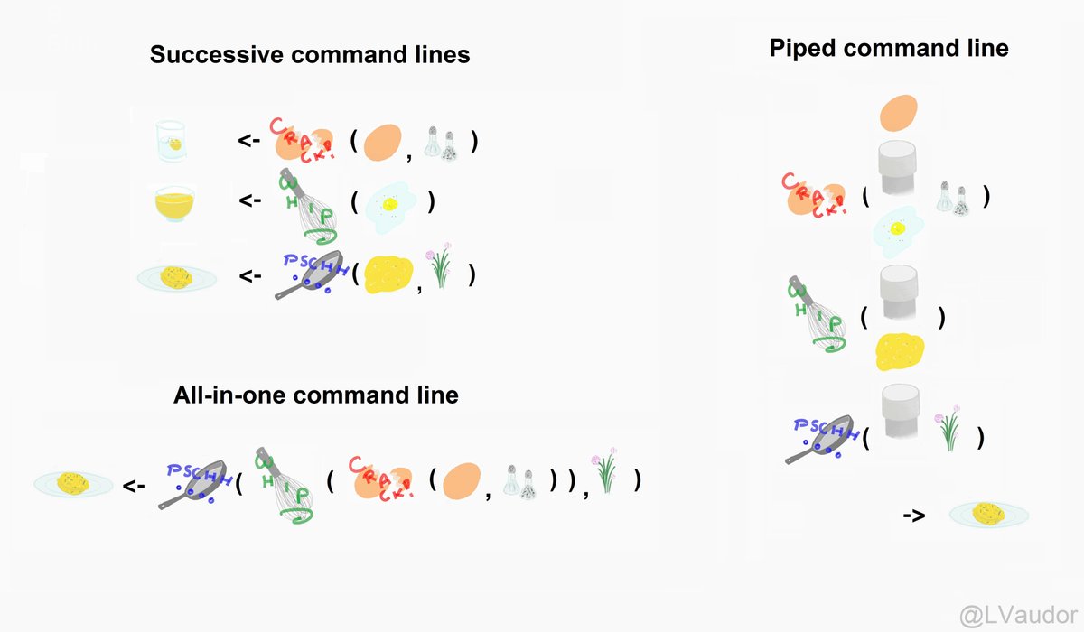

This is the idea behind a data pipeline.

`|>` or `%>%`?

You may encounter another pipe in R code:

%>%

For example:

recordTable %>%
  filter(Species == "White-tailed deer") %>%
  count(Station)

This pipe comes from the tidyverse ecosystem and was widely used before R introduced its own pipe:

|>

Both are still common.

In this course, we will primarily use:

|>

because it is now built directly into R.

Tip

You do not need to rewrite old code just because it uses %>%.

It is useful to recognize both.

For most of what we do in this course, they behave very similarly.

Putting everything together

Now let’s create a more complete pipeline.

Suppose we want to answer:

At how many stations was each of the five most commonly recorded species detected, and how many records did each species have?

First, define the species we want:

common_species <- c(
  "White-tailed deer",
  "Armadillo",
  "Racoon",
  "Hog",
  "Virginia opossum"
)

Then:

common_summary <- recordTable |>
  filter(
    Species %in% common_species
  ) |>
  group_by(Species) |>
  summarise(
    records = n(),
    stations = n_distinct(Station),
    total_individuals = sum(
      N_individuals,
      na.rm = TRUE
    ),
    .groups = "drop"
  ) |>
  arrange(
    desc(records)
  )

Look at the result:

common_summary

# A tibble: 5 × 4
  Species           records stations total_individuals
  <chr>               <int>    <int>             <dbl>
1 White-tailed deer    1266       16              1366
2 Armadillo             554       15               576
3 Racoon                522       11               538
4 Hog                   454       11               574
5 Virginia opossum      295        9               299

A relatively large raw dataset has now become a small table that directly answers our question.

From data manipulation to visualization

Because dplyr and ggplot2 are designed to work together, we can easily visualize our summarized data.

ggplot(
  common_summary,
  aes(
    x = Species,
    y = records,
    fill = Species
  )
) +
  geom_col(
    show.legend = FALSE
  ) +
  coord_flip() +
  labs(
    title = "Camera-trap records of common species",
    x = "Species",
    y = "Number of records"
  ) +
  theme_bw()

Notice that here we use:

geom_col()

instead of:

geom_bar()

Why?

geom_bar() counts the observations for us.

But common_summary already contains a column called:

records

with the counts we want to plot.

geom_col() uses those existing values directly.

From raw data to a result

At this point, we can begin to see a complete R workflow:

raw data
    ↓
import
    ↓
inspect
    ↓
filter / select
    ↓
create variables
    ↓
group and summarize
    ↓
visualize
    ↓
export

For example, we can save our species summary:

write_csv(
  common_summary,
  "outputs/common_species_summary.csv"
)

Now our entire workflow can be reproduced by running the script again.

Practice at home

Tip

This activity should take approximately 20–30 minutes.

Open your intro-r-course project and create:

practice-07.R

inside your scripts folder.

Load tidyverse and import:

data/recordTable.csv

Part 1: Select

Create a new object called:

practice_records

containing only:

Station
Species
N_individuals
Age
n_images

Part 2: Filter

Using practice_records:

Keep only "White-tailed deer" records.
Keep only records with more than one individual.
Try combining both conditions.

Part 3: Count

Using the original recordTable, calculate the number of records for each species.

Sort the result from most to least common.

Part 4: Group and summarize

Create one table with one row per Station.

For each station calculate:

number of records
number of species
total number of individuals

Part 5: Create a pipeline

Create a single pipeline that:

starts with recordTable,
keeps only "Armadillo", "Racoon", and "Hog",
keeps only records with N_individuals > 0,
groups by Species,
calculates the number of records,
calculates the number of camera stations,
sorts the table from the most to the fewest records.

Introduction

What is the tidyverse?

Let’s get started

Think of dplyr as a set of verbs

Selecting columns with select()

Removing columns

Selecting by data type

Filtering rows with filter()

Filtering numeric values

Multiple filtering conditions

Missing values

Sorting rows with arrange()

Renaming columns

Creating new columns with mutate()

Counting observations

Counting combinations

Unique values with distinct()

Grouping and summarizing data

More than one summary

Summarizing by camera station

Pipes

Why use pipes?

|> or %>%?

Putting everything together

From data manipulation to visualization

From raw data to a result

Practice at home

Part 1: Select

Part 2: Filter

Part 3: Count

Part 4: Group and summarize

Part 5: Create a pipeline

Think of `dplyr` as a set of verbs

Selecting columns with `select()`

Filtering rows with `filter()`

Sorting rows with `arrange()`

Creating new columns with `mutate()`

Unique values with `distinct()`

`|>` or `%>%`?