Objects, Data Structures, and Importing Data

Session 2

Gabriel Andrade

Objects, Data Structures, and Importing Data

Session 2

Today we will connect three important ideas:

objects → data structures → external data files

By the end, we should be able to create simple R objects, understand the basic structure of datasets, and import data from CSV and Excel files.

R works with objects

Most of the time, we give R a value and store it in an object.

number_of_cameras <- 12

species <- "Raccoon"

camera_active <- TRUE

The object name is on the left.

The value is on the right.

object_name <- value

Why create objects?

Without an object, R gives us a result but does not save it.

2 + 2

But if we assign the result:

result <- 2 + 2

we can use it again later.

result
result * 10

Objects allow us to build an analysis step by step.

Naming objects

Good object names make code easier to understand.

x <- 25

works, but this is more informative:

number_of_cameras <- 25

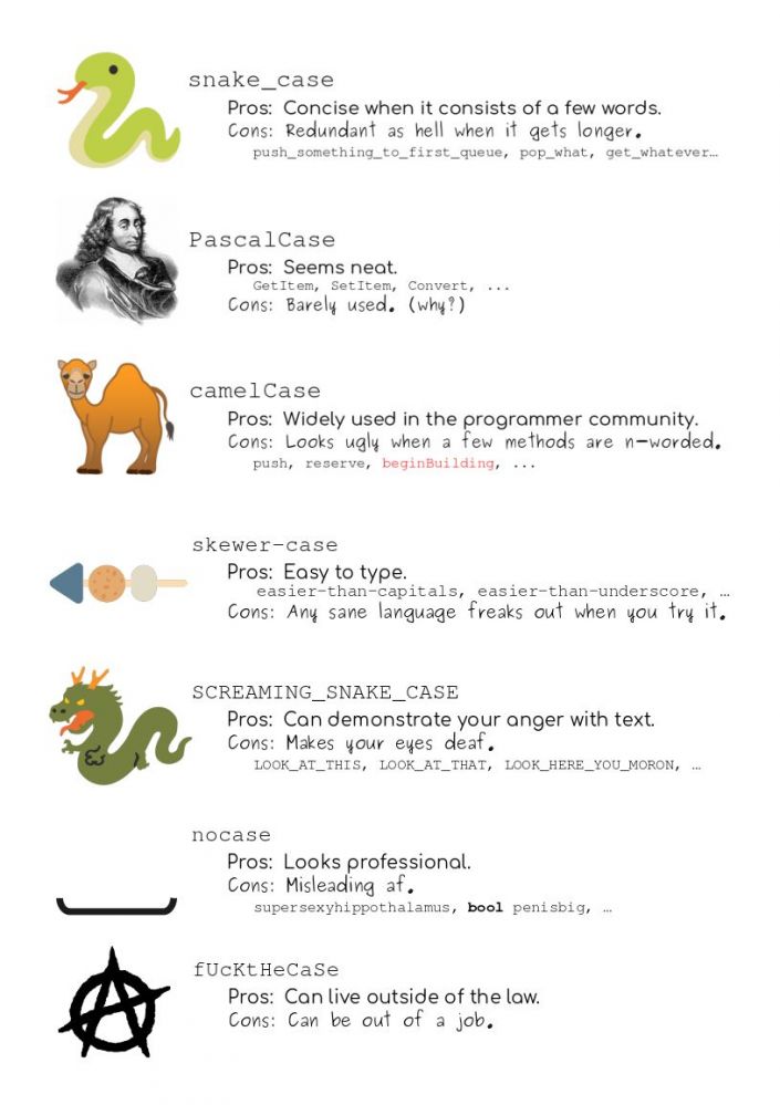
During this course, we will mostly use snake_case.

camera_days
number_of_detections
survey_data

A few naming rules

Object names:

should not begin with a number
should not contain spaces
should avoid special characters
should avoid accents
should not reuse common function names

R is case-sensitive:

camera_data
Camera_data

are different names.

Basic object types

R can store different types of values.

Type	Example
numeric	`25`
character	`"Raccoon"`
logical	`TRUE`
missing value	`NA`

A number inside quotation marks is not a number.

fake_number <- "25"

Operators

Arithmetic operators return numbers.

Relational operators return TRUE or FALSE.

10 > 5
10 == 5
10 != 5

Functions

Functions perform specific tasks.

Most functions look like this:

function_name(object)

For example:

class(25)
class("25")
class(TRUE)

Functions can also use arguments:

round(3.14159, digits = 2)

Help is part of using R

You do not need to memorize every function.

Use the help system:

or:

Learning R is not memorizing commands.
It is learning how to find what you need.

Packages

Many functions come from packages.

The basic workflow is:

install → load → use

For example:

#| eval: false
#| 
install.packages("beepr")

library(beepr)

beep(sound = 8)

Code-along 1

Switch to RStudio.

Create a script called:

session-02.R

inside your scripts/ folder.

Then create:

species <- "Raccoon"
station <- "CT01"
detections <- 15

Use R to ask:

detections > 10
class(species)
class(detections)

From single values to data structures

So far, most objects had one value.

Real datasets have many values.

R can organize values into different structures:

vectors
matrices
lists
data frames

For this course, data frames will be the most important.

Vectors

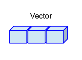
A vector stores several values in one object.

detections <- c(5, 12, 8, 0, 3)

The function c() means combine.

We can use functions on vectors:

mean(detections)
sum(detections)
length(detections)

Vectors have one data type

A vector can contain numbers:

camera_days <- c(30, 28, 30, 25)

or text:

species <- c("Raccoon", "Coyote", "Bobcat")

or logical values:

camera_active <- c(TRUE, TRUE, FALSE)

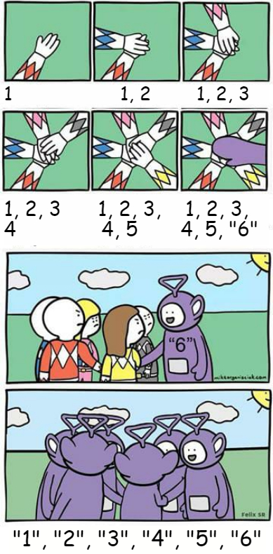
But mixing types can change the result.

mixed_vector <- c(1, 2, "Raccoon", 4)
class(mixed_vector)

Selecting values from vectors

Use square brackets:

detections <- c(5, 12, 8, 0, 3)

detections[1]
detections[3]
detections[1:3]
detections[c(1, 3, 5)]

R starts counting at 1.

Selecting with conditions

Relational operators work with vectors.

detections > 5

This returns one logical value for each element.

We can use that condition to select values:

detections[detections > 5]

This is the basic idea behind filtering data.

Matrices

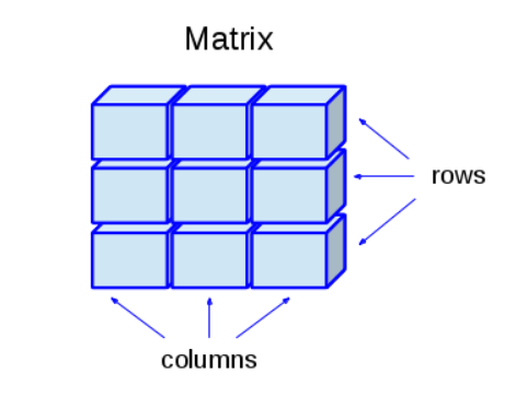
A matrix has two dimensions:

rows × columns

Example:

detection_matrix <- matrix(
  1:12,
  nrow = 4,
  ncol = 3
)

detection_matrix

To select values:

detection_matrix[row, column]

Why should we care about matrices?

Camera-trap detection histories often look like matrices.

        occasion_1  occasion_2  occasion_3
CT01         0           1           0
CT02         1           0           0
CT03         0           0           1

Rows are sites or stations.

Columns are sampling occasions.

Lists

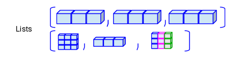
Lists can store different kinds of objects together.

camera_information <- list(
  station = "CT01",
  active = TRUE,
  detections = 25,
  species = c("Raccoon", "Coyote", "Bobcat")
)

Access elements with:

camera_information$station
camera_information$species

Many R functions return lists.

Data frames

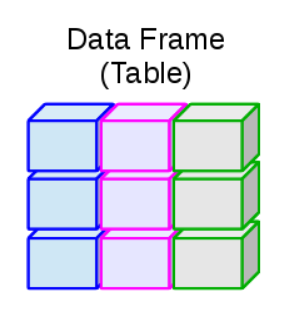
A data frame is a rectangular table.

It has:

rows
columns

It looks similar to an Excel spreadsheet.

But unlike a matrix, each column can have a different type.

Data frames

Creating a data frame

station <- c("CT01", "CT02", "CT03", "CT04")

habitat <- c("Forest", "Forest", "Pasture", "Pasture")

camera_days <- c(30, 28, 30, 27)

active <- c(TRUE, TRUE, FALSE, TRUE)

camera_data <- data.frame(
  station,
  habitat,
  camera_days,
  active
)

camera_data

Rows and columns

In most ecological datasets:

rows    = observations
columns = variables

For example:

station	habitat	camera_days	active
CT01	Forest	30	TRUE
CT02	Forest	28	TRUE
CT03	Pasture	30	FALSE

Each row is one camera station.

Each column is one variable.

Inspecting data frames

Before analyzing data, inspect it.

head(camera_data)
str(camera_data)
dim(camera_data)
names(camera_data)

Ask:

How many rows?
How many columns?
Are the column names correct?
Are numeric columns actually numeric?

Selecting from a data frame

Use $ to select a column:

camera_data$station
camera_data$camera_days

Use [row, column] to select by position:

camera_data[1, 2]
camera_data[1, ]
camera_data[, 2]

Later we will learn more readable tools with dplyr.

Code-along 2

Create this data frame:

station <- c("CT01", "CT02", "CT03")

habitat <- c("Forest", "Pasture", "Forest")

detections <- c(12, 5, 0)

survey_data <- data.frame(
  station,
  habitat,
  detections
)

Then run:

survey_data
str(survey_data)
survey_data$detections

External data files

Most real data will not be typed directly into R.

They will usually come from:

Excel
Google Sheets
field-data software
camera-trap metadata
another program

So R needs to know where the file is.

Working directory

The working directory is the folder where R starts looking for files.

Check it with:

getwd()

Because we are using an RStudio Project, the working directory should be the main project folder.

intro-r-course/

Relative paths

If your file is here:

intro-r-course/
│
├── data/
│   └── camera_data.csv
│
├── scripts/
└── outputs/

you can refer to it as:

data/camera_data.csv

This is better than using a full path from your own computer.

CSV files

CSV means:

Comma-Separated Values

A CSV is a plain-text table.

station,species,detections,camera_days
CT01,Raccoon,12,30
CT02,Coyote,5,28
CT03,Bobcat,8,30

CSV files are simple, portable, and easy to read in R.

Importing a CSV file

Base R:

camera_data <- read.csv("data/camera_data.csv")

Tidyverse / readr:

library(tidyverse)

camera_data2 <- read_csv("data/camera_data.csv")

The important pattern is:

object <- read_function("path/to/file")

Importing Excel files

To read Excel files, use readxl.

library(readxl)

camera_data3 <- read_excel("data/camera_data.xlsx")

If the file has multiple sheets:

excel_sheets("data/camera_data.xlsx")

camera_data3 <- read_excel(
  "data/camera_data.xlsx",
  sheet = "camera_records"
)

Always inspect imported data

After importing:

head(camera_data)
str(camera_data)
dim(camera_data)
names(camera_data)

Do not assume the file imported correctly just because R did not show an error.

Trust, but verify.

Common import problems

Most import errors are simple:

wrong file name
wrong folder
different capitalization
missing package
file not saved in the project
Excel changed dates or values

Useful checks:

file.exists("data/camera_data.csv")
list.files("data")

Code-along 3

Download the example files from Module 4.

Place them in:

intro-r-course/data/

Then import the CSV:

camera_data <- read.csv("data/camera_data.csv")

Inspect it:

head(camera_data)
str(camera_data)
dim(camera_data)
names(camera_data)

Code-along 4

Now import the Excel file.

library(readxl)

camera_data_excel <- read_excel(
  "data/camera_data.xlsx"
)

Check the sheets:

excel_sheets("data/camera_data.xlsx")

Inspect the object:

head(camera_data_excel)
str(camera_data_excel)

Exporting data

To save a CSV from R:

write.csv(
  camera_data,
  "outputs/camera_data_clean.csv",
  row.names = FALSE
)

With readr:

write_csv(
  camera_data,
  "outputs/camera_data_clean.csv"
)

Keep raw data separate

A useful structure:

intro-r-course/
│
├── data/
│   └── camera_data.csv
│
├── scripts/
│   └── session-02.R
│
└── outputs/
    └── camera_data_clean.csv

data/ contains original or input files.

outputs/ contains files created by your analysis.

Practice at home

Before the next session:

Open your intro-r-course project.
Create practice-02.R and practice-03.R if you have not done them yet.
Download the Module 4 example CSV and Excel files.
Import both files into R.
Inspect them using:

head()
str()
dim()
names()

Export one CSV file into the outputs/ folder.

Main idea

R work often follows this pattern:

create objects
      ↓
organize values
      ↓
import data
      ↓
inspect data
      ↓
work with data
      ↓
export results

The details take practice.

But this workflow will appear again and again.